How To Make an Attendance Sheet in Excel (Free Template Included)

To run payroll accurately and stay compliant, you need accurate attendance data. An Excel attendance tracking spreadsheet is a simple solution—but only if you set it up correctly. 

This guide will give you practical steps (with lots of visuals) to get you from “Untitled spreadsheet.xls” to “Attendance Sheet – final.xls.” You can also download our free, ready-to-use employee attendance tracker template!

What Is an Attendance Sheet? 

An attendance sheet is a physical or digital document that tracks employees’ attendance status during shifts or other work events. 

It lists your team members’ names, whether they were present or absent, the department/team, and the attendance timeframe (e.g., day, week, month). 

What Do You Use an Attendance Sheet For?

You use an attendance sheet to track and calculate the days when employees are present or absent. Depending on your HR needs, you might further break down absences into sick days, no-call no-shows, and leave types such as parental, compassionate, and vacation.

An accurate attendance tracking spreadsheet helps you:

• Quickly calculate employee payroll, including sick pay.
• Stay legally compliant with state and federal employment laws, such as those mandating paid and unpaid leave.
• Detect absenteeism before it impacts your labor costs and team morale.

Attendance sheets come in many formats, including pen-and-paper, physical spreadsheets, digital spreadsheets, and employee attendance app reports. 

How to Make an Attendance Sheet in Excel

Tracking employee attendance in Excel doesn’t have to be rocket science. To prove it, we’re giving you two options:

Option A: Use our ready-made Excel template
Option B: Create your own Excel attendance sheet from scratch

Let’s break them down below. 

Option A: Use Our Ready-Made Attendance Sheet Template

First, download and open our expert-vetted Excel attendance sheet template.

Next, adjust it to your needs using the following steps:

Step 1: Adjust the month and days

• Replace “October 2024” in cell A6 with the month and year you’re tracking.
• Clear row 8. Right-click on row 8 (at the far left), then select “Clear Contents.”
• Clear the columns containing the dates 29, 30, and 31, depending on the month. To do this, right-click on the column (e.g., column AL) and select “Clear Contents.”
• Add the first three letters of the weekday in H8, above “1”  (e.g., Mon, Tue, Wed) corresponding to the 1st of the month. Then, click the tiny square in the bottom-right corner of the same cell and drag it across row 8 until you reach the last date. The row should now be filled with three-letter weekdays for the entire month.

Step 2: Add employee details

• Select all cells under the column header “Employee Name” (in this case, A10-A19). Press the Delete key on your keyboard.
• Enter your employees’ names manually or copy and paste the list from a different source (such as a payroll report). 

Step 3: Add your brand

• Add your logo. Click on cell A1 (*Add your company logo here*) and hit the Delete key on your keyboard. Click “Insert” on your Excel menu, then the Pictures icon in the “Illustrations” category, then “This Device.” Open the folder containing your company logo, or download it first if you haven’t already. Select the image and click “OK.”
• Fill column headers with your brand colors. First, have your brand color’s HEX or RGB code handy. (Ping your marketing team for this, or use a code picker like imagecolorpicker.com to get the codes.) Then, click the arrow next to the fill color icon under “Fonts,” click “More colors,” select “Custom,” add your HEX/RGB code, and click “OK.” Or, more simply, pick a standard color that most resembles your brand color! Finally, drag your cursor to select all the table headers and press the color fill icon.

Presto! Your Excel attendance tracking spreadsheet is now ready to go.

Option B: Make Your Own Attendance Sheet for Employees

Building an Excel attendance sheet from scratch gives you the know-how to make sheets for different projects, teams, and HR needs. 

As you follow our steps below, you can personalize your sheet—for instance, by adding an “Employee ID” column or separating staff first names from last names.

Here’s a simple, step-by-step guide to help you build your sheet in your Excel workbook.

Step 1: Set up your sheet 

Let’s start with the sheet structure.

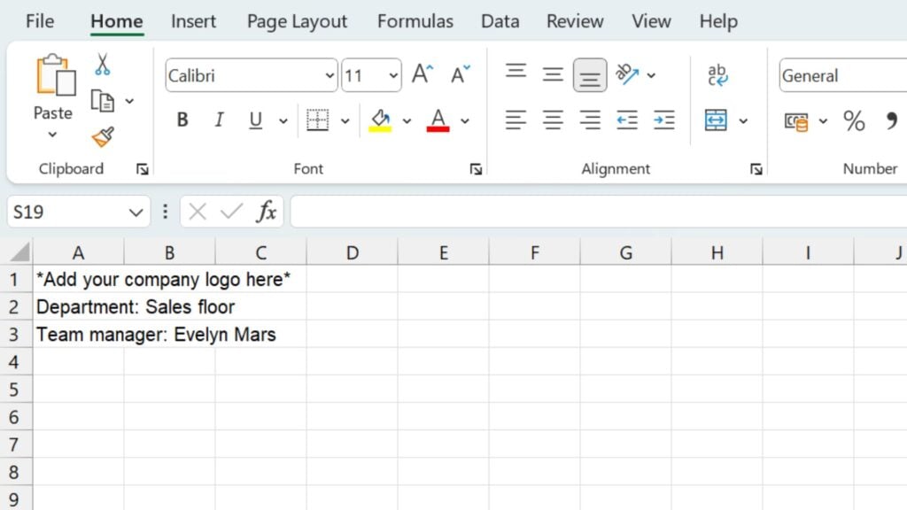
In the top left, spare the first three rows for useful info like your company name and the department and team manager linked to the attendance sheet. Add the following:

• Your company name in A1 or a logo image (click the “Insert” tab, “Illustrations,” “Pictures,” then “This Device.” Choose the image and click OK.) 
• Department: [name of department] in cell A2
• Team manager: [name of team manager] in cell A3

Next, add a title to the worksheet:

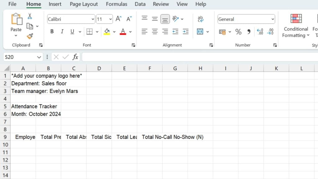
• Add “Attendance Tracker” in cell A5. 
• Add “Month: [Month Year]” in cell A6. 

Then, you’ll add headings to the attendance summary table, which sits on the left-hand side of the sheet. Insert the following texts in individual cells from A9 to F9:

• Employee Name
• Total Present (P)
• Total Absent (S+L+N)
• Total Sick Days (S)
• Total Leave (L)
• Total No-Call No-Show (N)

Next, you’ll set up the monthly attendance tracking table on the right-hand side of the sheet. Depending on the month, this table will have between 28 and 31 entries for each employee. If you have, say, 10 staff members, your monthly attendance table will be 10 rows long and between 28 and 31 columns wide (excluding headers). 

Let’s begin:

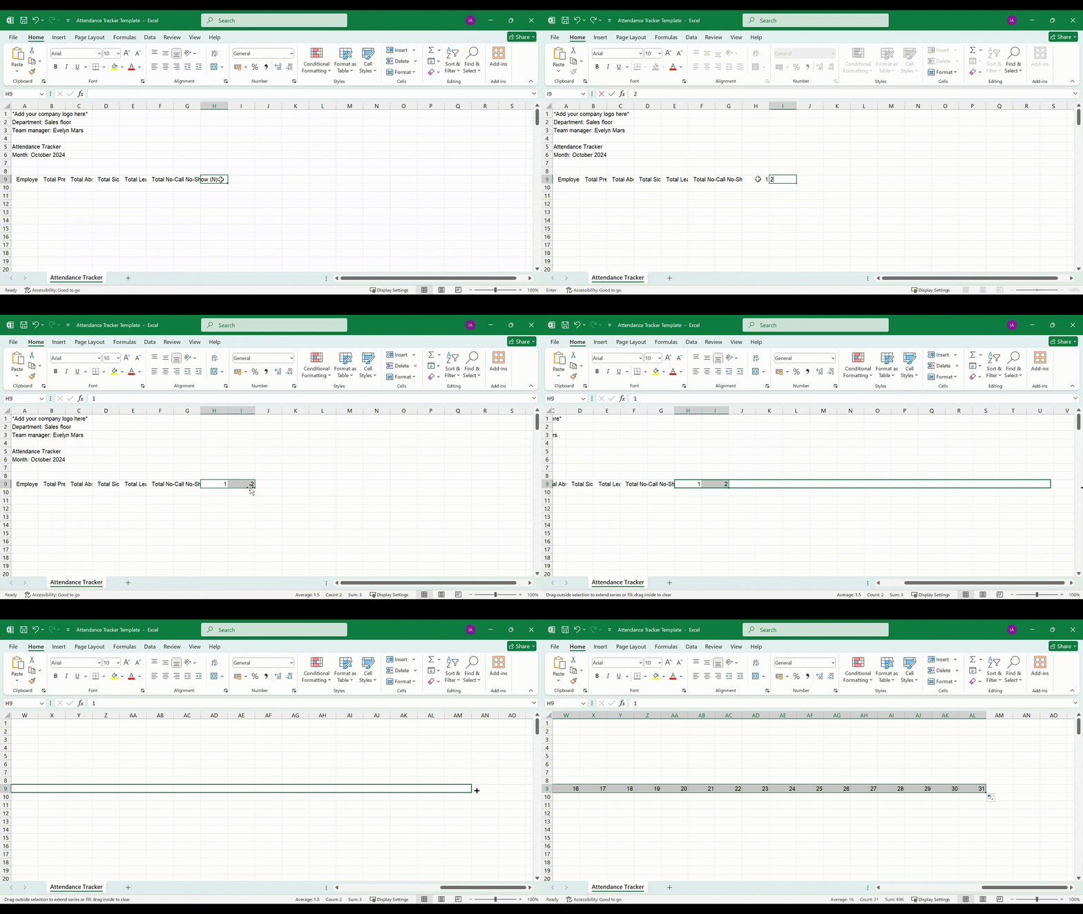
• Add number-only dates (i.e., 1, 2, 3, etc.) to each cell from H9 to the right, ending with the last day of the respective month (e.g., 31 for October). To speed things up, add “1” in H9 and “2” in I9. Then, select these two cells, click the tiny square at the bottom right corner of the highlight, and drag it to the right for another 29 cells. All 31 dates should now be filled in.

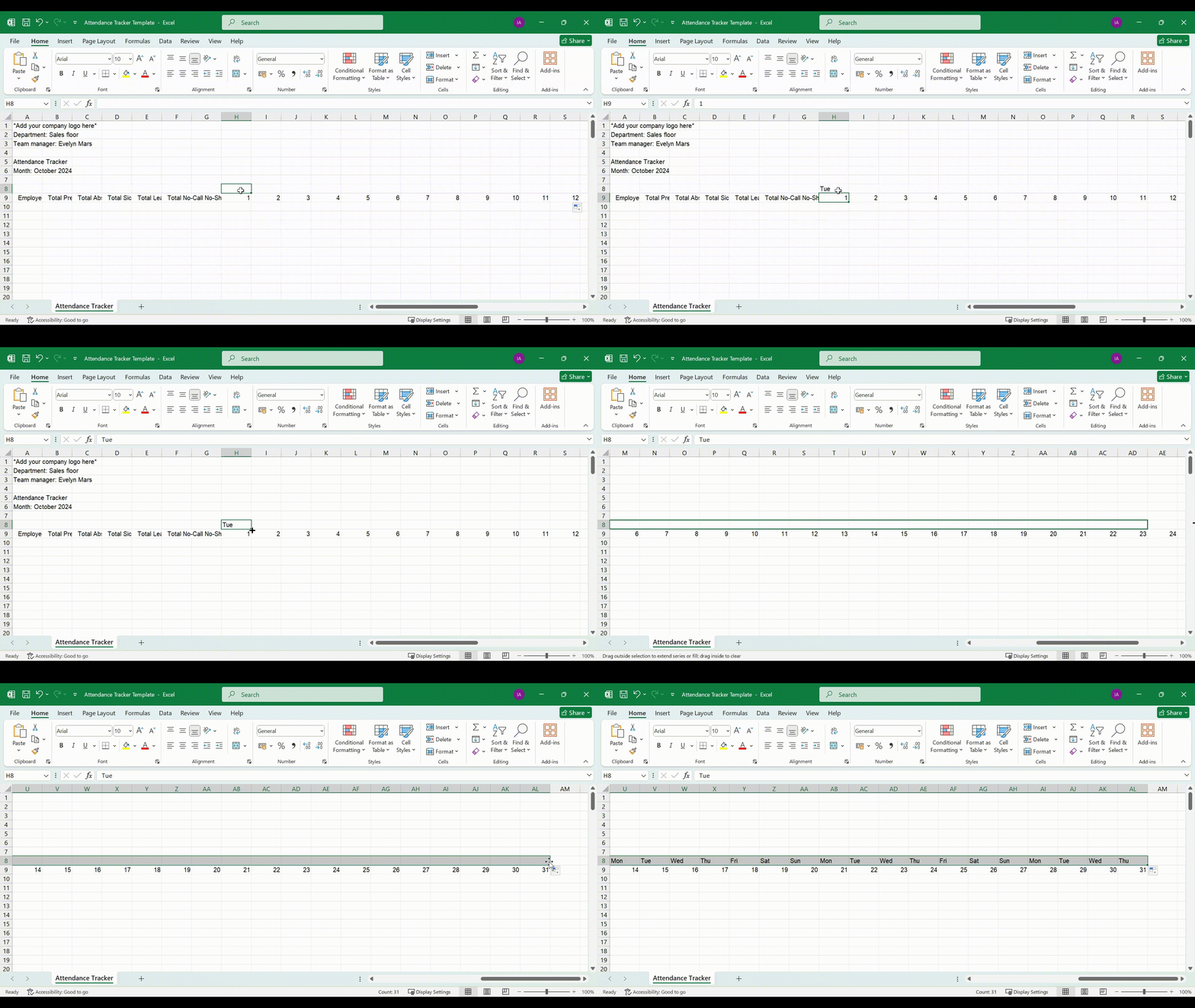
• Add three-letter weekdays (i.e., Mon, Tue, etc.) above the dates you just added. Check what day your month starts on—for October 2024, it’s Tuesday. In this case, write “Tue” in H8, click on the tiny square in the bottom right corner, and drag to the right until you reach the 31st. Weekdays should now be filled in across the month.

Finally, some design changes will help you navigate the sheet more easily:

• Bold rows 1 to 9.
• Resize the font in cell “Attendance Tracker (A5) to 24.
• Resize the font in cell “Month: October 2024” to 12.

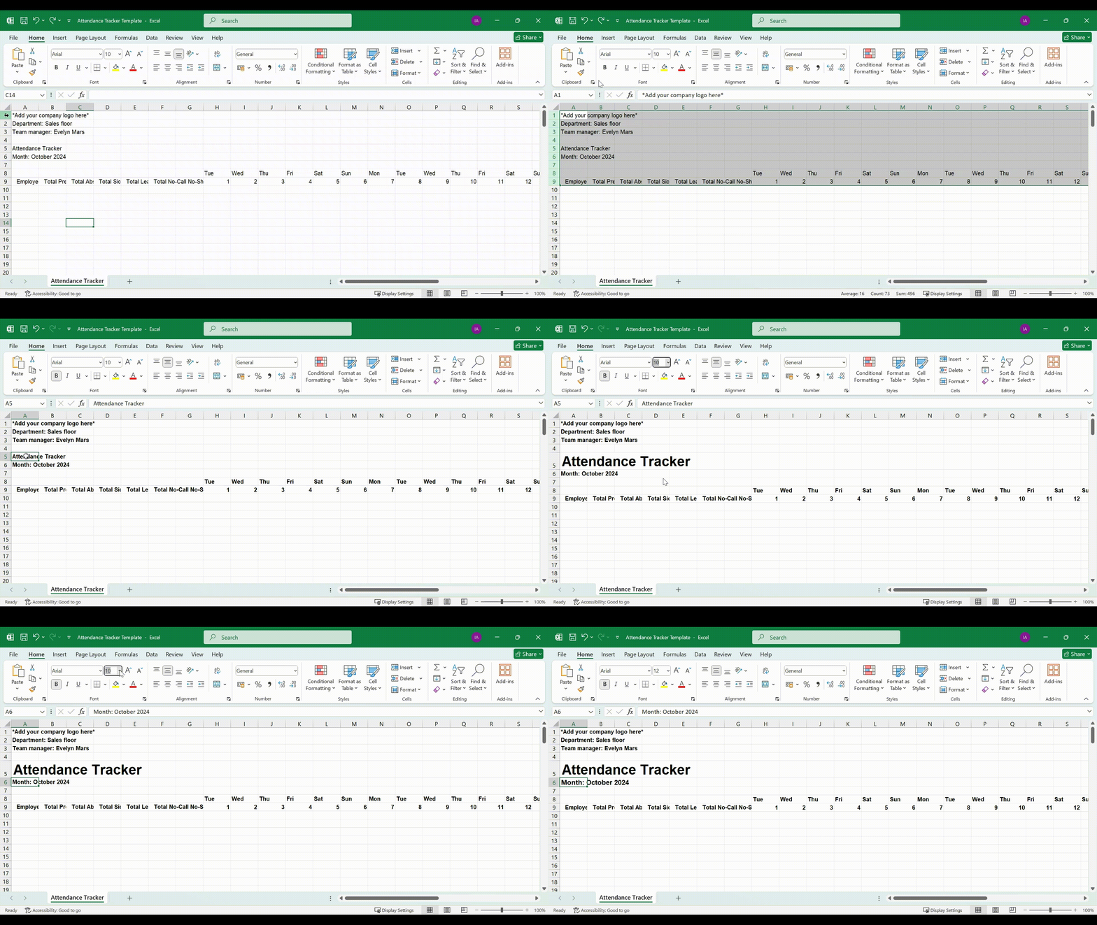
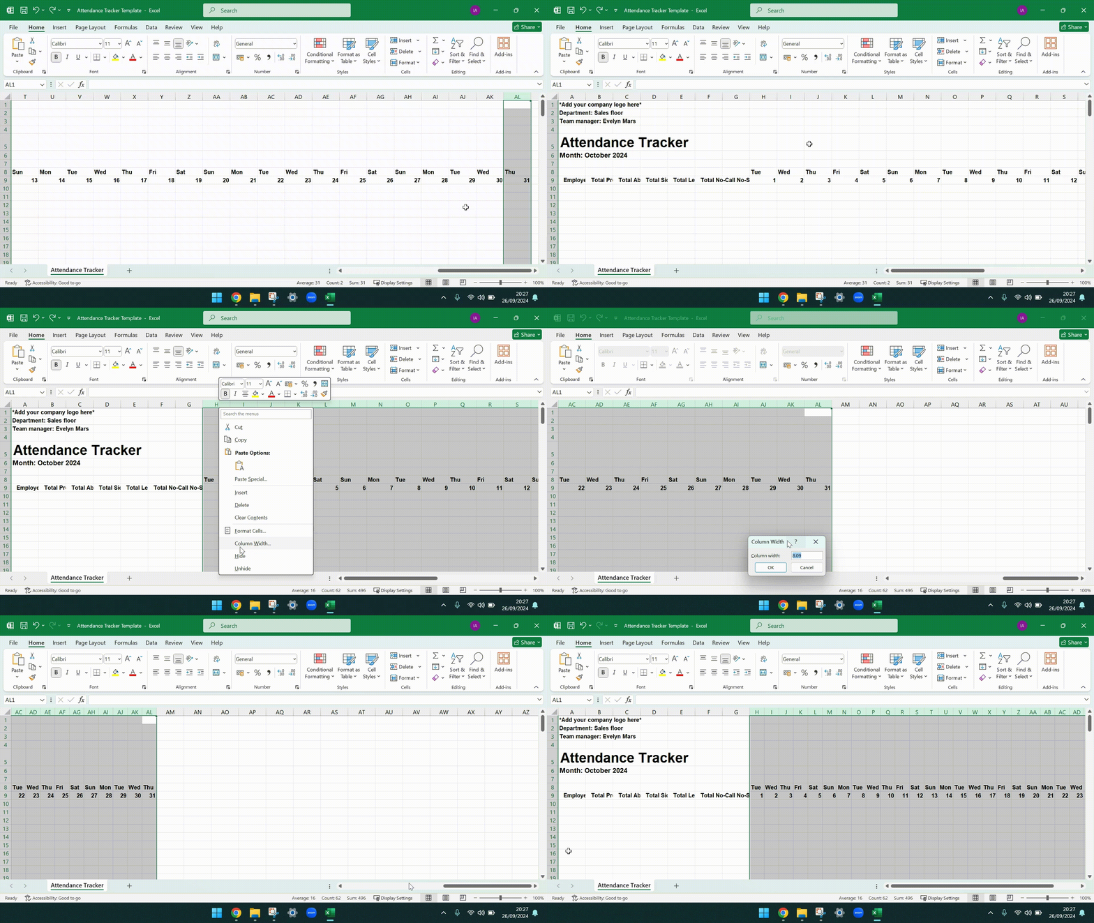
• Resize all columns from H to AL to width 30. Do this by clicking column H (at the top), holding the Shift key, then clicking column AL. With this range highlighted, right-click on any column and, in the dropdown, select “Resize columns.” Under “Enter new column width,” type in 4, then click “OK.”

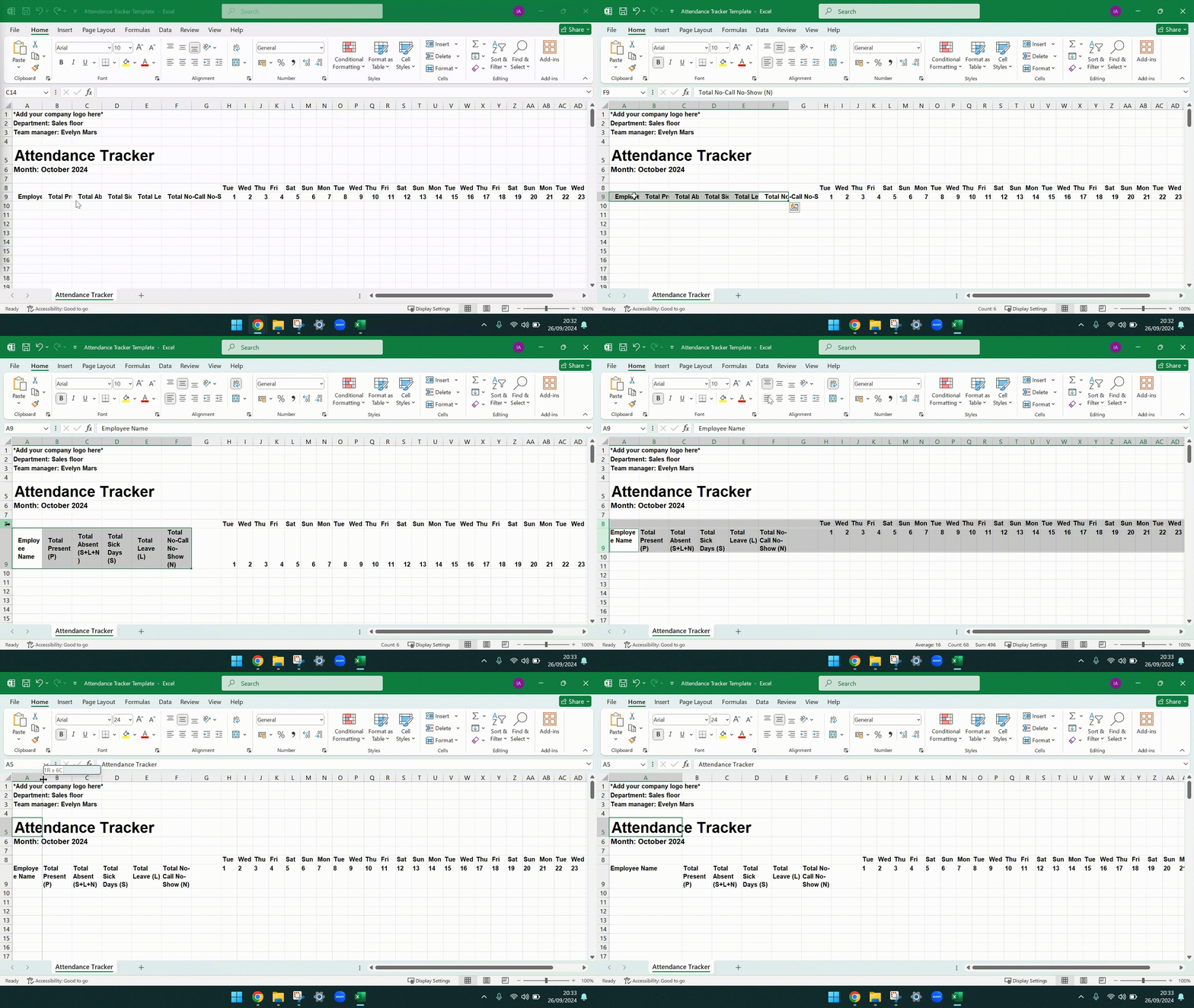
• Wrap the summary table header cells. Select the headers (A9-F9), then click the wrap text icon in the Home toolbar.
• Select top-left vertical alignment for rows 8 and 9. Click on row 8 (at the far left), hold the Ctrl key, then click row 9. Tap the top icon for vertical alignment and the left icon for horizontal alignment. Both icon types are in the “Alignment” section.
• Expand individual rows and columns to increase text visibility where required (mainly for A9-F9).

Step 2: Add employees’ names

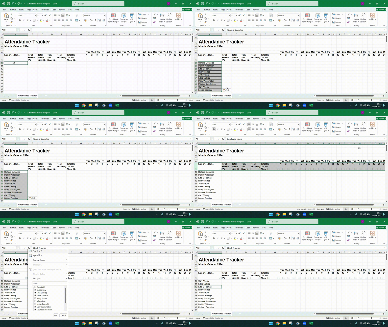
Fill in your employees’ full names in individual cells from A10 downward. (For instance, if you’re adding 10 employees, the last name will be in cell A19.)

Step 3: Include attendance labels

Next, set up a dropdown for attendance labels for each day. In our template, the options are P (Present), S (Sick day), L (Leave), and N (No-call no-show). 

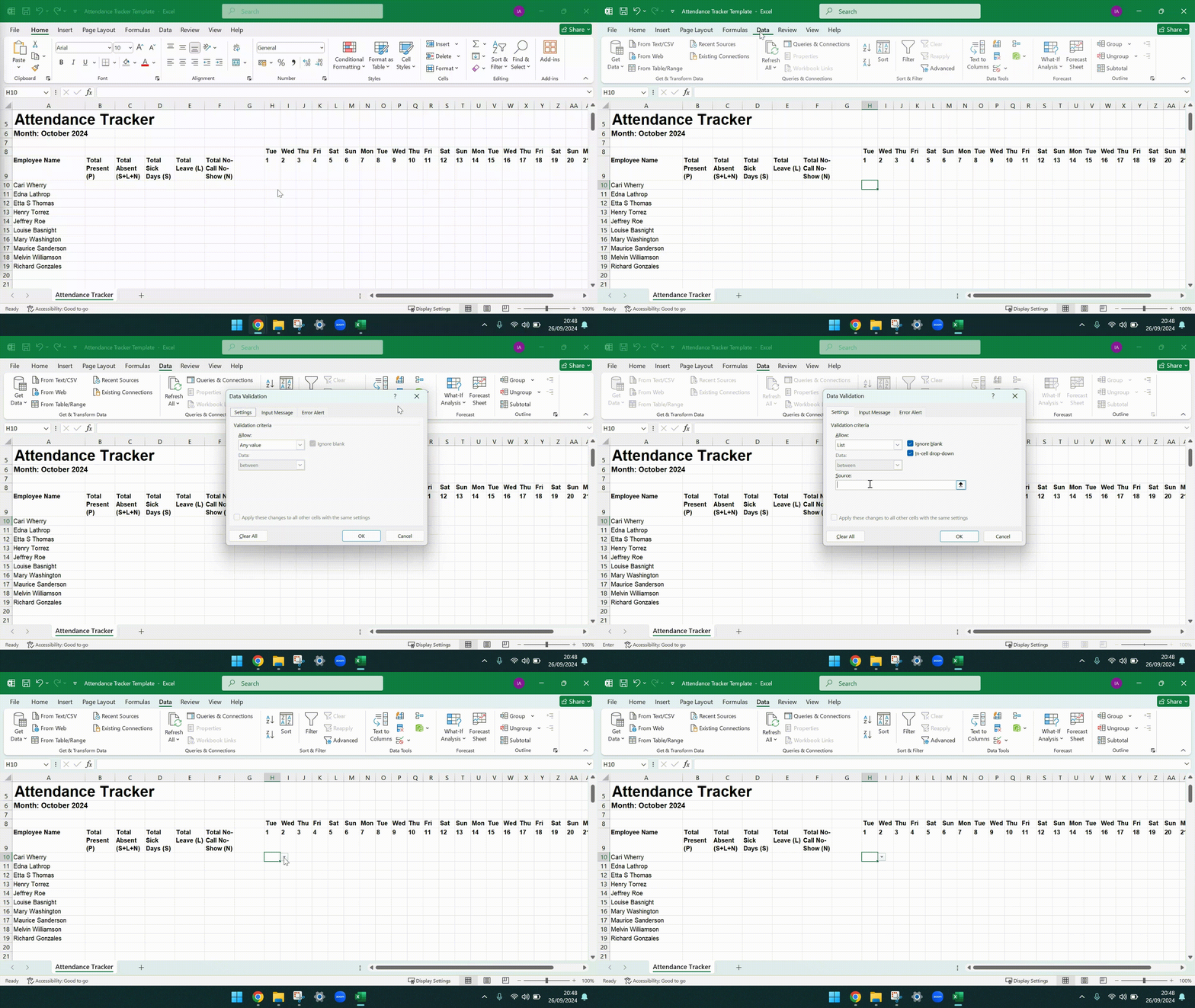
Select H10, click “Data” in the top menu, then click the “Data Validation” icon. In the box under “Settings” click “Allow: List.” Then, under Formula, write the four values separated by commas: P, S, L, N.

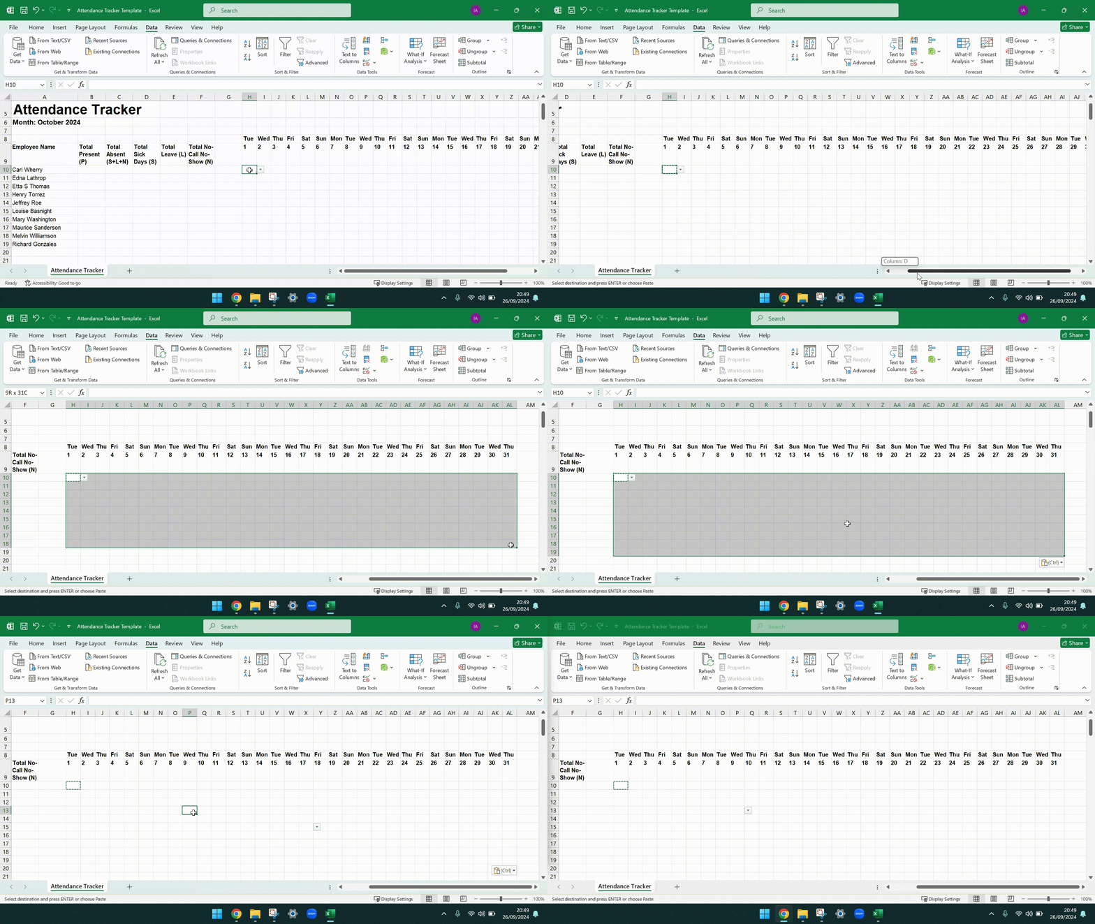
To apply this data validation rule across the tracker, copy the cell you just validated (H10), select the entire table (H10-AL19), and paste the empty cell. The dropdown should now be available on every date for every employee.

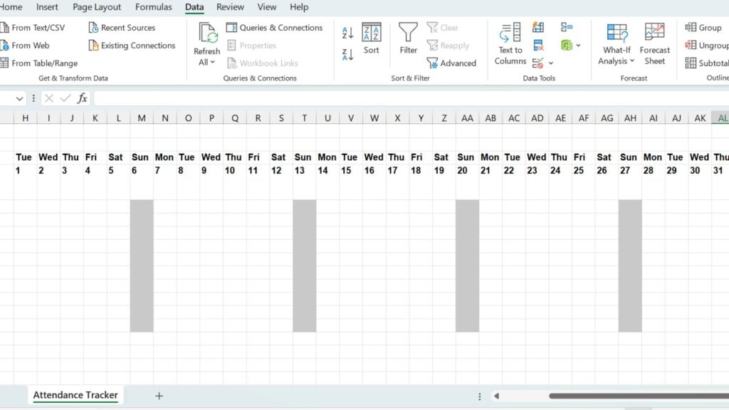
Now, gray out any days when your business or team doesn’t operate, such as weekends or public holidays. As an illustration, we grayed out Sundays.

Step 4: Add conditional formatting to the tracker

Next, add some color coding to your employee attendance tracker using conditional formatting. That way, whoever is glancing at it can quickly understand whether there’s good attendance, a lot of sick leave, etc.

To keep it simple, automate only the cell fill color depending on the attendance labels P, S, L, and N. Here’s how:

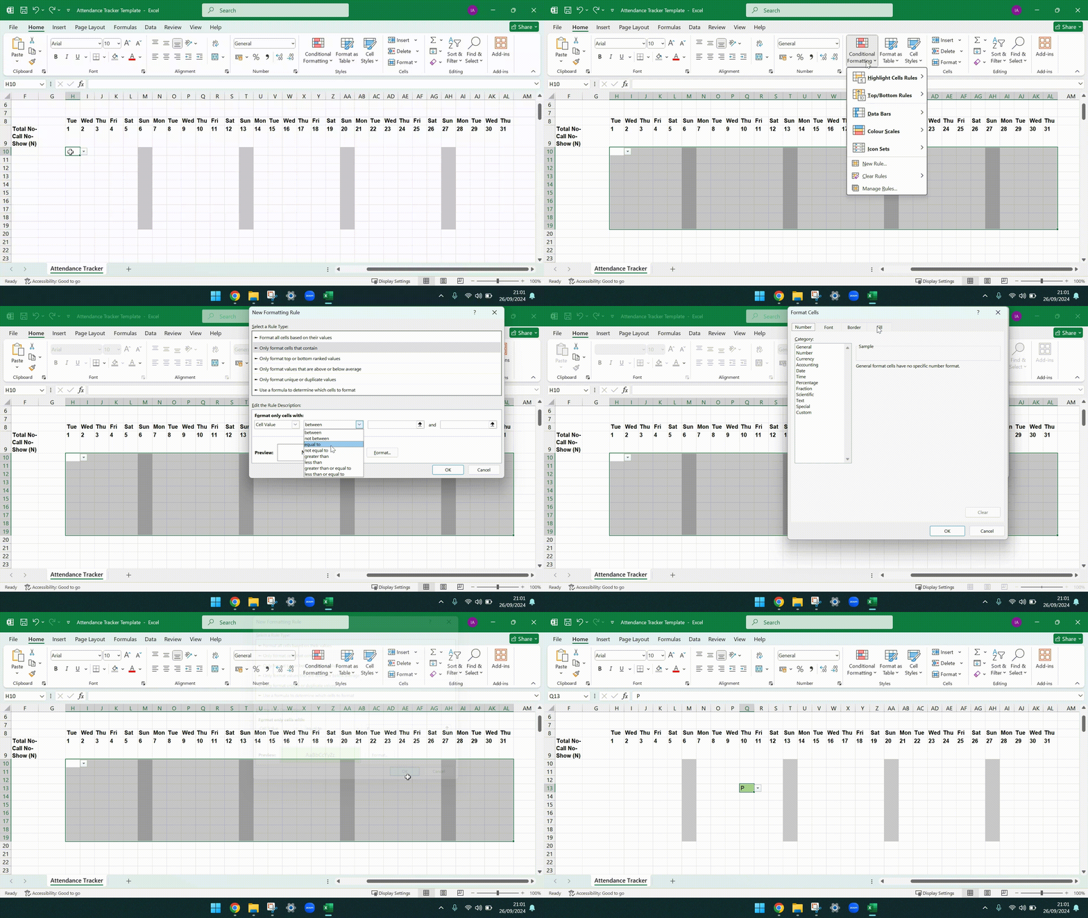
• Select the whole table range, excluding headers (H9-AL19).
• In the Home toolbar, click “Conditional Formatting” > “New Rule.”
• Pick “Only format cells that contain.”
• Under Edit the Rule Description, select the following:
  • Cell Value equal to “P”
• Click “Format” below, select the Fill tab, and pick a color to go with “Present.” (Green, perhaps?) 
• Click “OK.”
• Repeat the above steps for the remaining attendance labels, choosing different fill colors. (How about orange, blue, and red?)

To test that it’s working, change one of the attendance sheet cells to “P.” Did the fill color change? Great! 

Step 5: Calculate totals per employee

Rather than manually calculate the total present or absent days per employee, pop the tracking table into a few formulas. That’s what the summary table on the left is for.

To add formulas, double-click a cell and write in the formula bar (the white strip just below the top toolbar). 

We wrote the formulas for you based on the rows and columns outlined above. If you’ve made your own changes alongside, you may have to adjust the column letters or row numbers in the formulas to cover the whole area of your tracking table.

• In B10, under Total Present (P), paste:
  • =countif(H10:AL10,”P”)
• In C10, under Total Absent (S+L+N), paste:
  • =sum(D10:F10)
• In D10, under Total Sick Days (S), paste:
  • =countif(H10:AL10,”S”)
• In E10, under Total Leave (L), paste:
  • =countif(H10:AL10,”L”)
• In F10, under Total No-Call No-Show (N), paste:
  • =countif(H10:AL10,”N”)

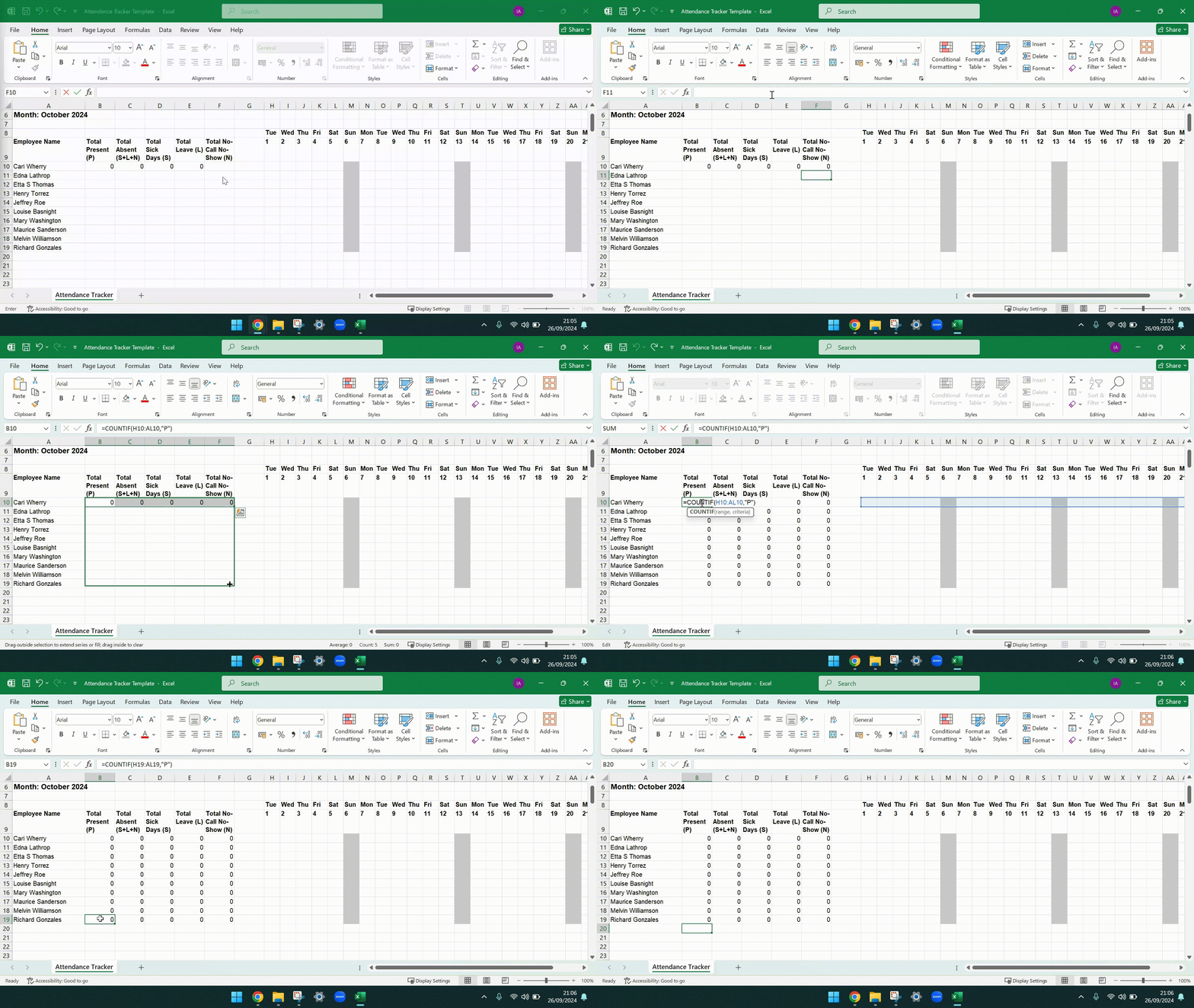
Once you have this down for the first row (i.e., the first employee), drag your cursor to highlight all the cells where you’ve just placed formulas. Then, pull the tiny square on the bottom right down to the last employee row. If you double-click any of the “Total Present (P)” formulas, for instance, you’ll see the tracker rows highlighted are on the same row as the formula.

Step 6: Add finishing touches ✨

You’ll use your attendance sheet more quickly and reduce the risk of errors when it’s neatly designed. So, remember to add these finishing touches:

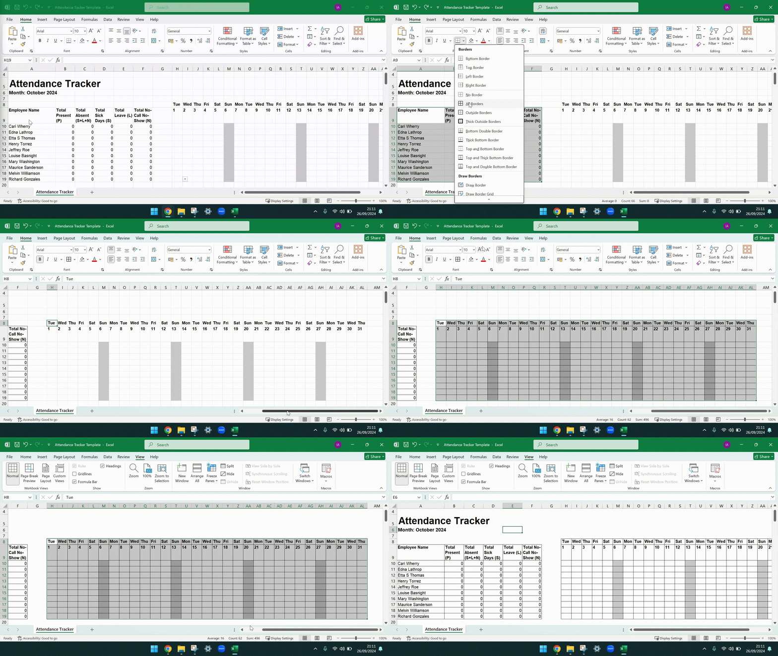
• Add table borders. First, select the left-hand side totals table (A9-F19). While it’s highlighted, click the arrow dropdown next to the border icon in the “Fonts” section of the “Home” tab. Then, select “All Borders.” Follow the same steps to border up the attendance tracking table on the right (H10-AL19).
• Hide gridlines. Optionally, for a sleek effect, click the “View” tab in the Excel menu. In the “Show” section, untick “Gridlines” if it’s currently ticked.

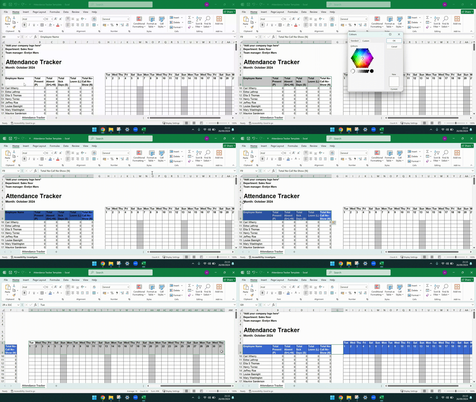
• Add your brand colors to the table headers. Once you have your brand color’s HEX or RGB code, select the table headers, click the arrow next to the “Fill Color” icon (in “Font”), select “More Colors,” then “Custom.” Paste in your code and click “OK.”

Step 7: Save your sheet

It’s obvious, we know. But we wouldn’t want you to put in all that hard work only to forget to save your sheet. Here’s how to do it:

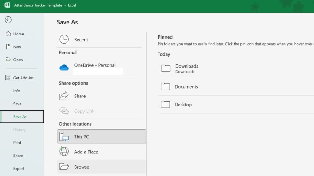
• Click the “File” tab, then “Save As,” then “Browse”. 
• In the pop-up window, select the folder you’re saving the sheet to. 
• Type in a clear file name (e.g., “Attendance Tracker – Sales Floor – October 2024”). 
• Hit “Save.”

Now you’re done!

Pros and Cons of Using Excel to Create Attendance Sheets

Here are the pros and cons of using Excel for attendance management:

👍 Pros	👎 Cons
Free with a Microsoft Office license	Costly in case of error (e.g., misspelling an employee’s name could be a legal liability)
Relatively easy to learn	Prone to error (e.g., an employee might accidentally edit a cell formula or forget to save changes)
Accessible from emails and mobile phones	Employees may not open the correct version of the attendance sheet
Real-time collaboration possible on cloud drives such as Microsoft 365	Version control can be difficult with multiple simultaneous edits
Customizable design, layouts, and formulas according to business needs	Linking the sheet data with other Excel trackers (e.g., vacation tracker) can be difficult with varying sheet setups
Easy to share with external collaborators such as accountants or HR consultants (with no sign-in required)	Data security risks if sensitive employee data is leaked

Simplify Attendance Tracking with Connecteam

Accurate attendance data helps you tackle absenteeism and stay compliant with labor laws. And, using either our downloadable template or our step-by-step instructions, building your own attendance spreadsheet in Excel is a piece of cake.

That said, Excel attendance trackers have downsides. From data security risks to manual errors and access mishaps, Excel sheets can become costly and time-consuming to manage, especially for growing teams. 

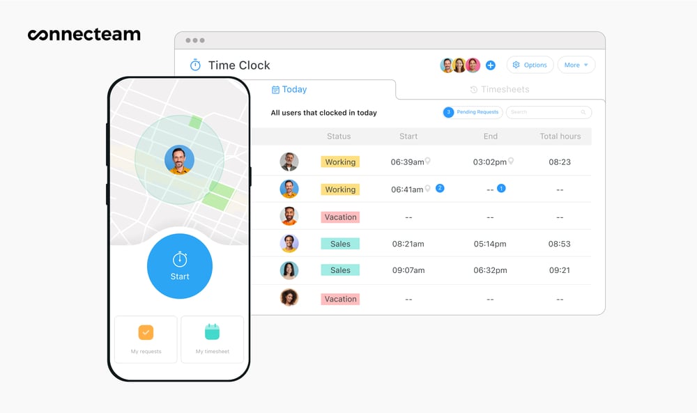
A secure and automated attendance tracking app can help. Connecteam is a leading workforce management solution that lets teams store employee data, build work schedules, clock in and out of shifts, and auto-generate timesheets—just in time for payroll. 

Connecteam has a fully functional mobile app (great for on-the-go employees) with geofencing features. With this, you can know both when and where your team is clocked into a shift.

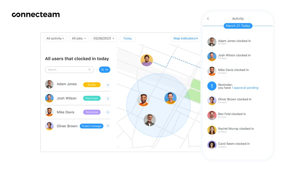
Plus, you can get notified when scheduled staff doesn’t clock in, accept time off requests with one tap, and view and download attendance reports on your phone or desktop.

In short, Connecteam is your go-to for attendance tracking (no formulas or conditional formatting required).

Give Connecteam a try for free today!

FAQs

How do I keep track of employees’ attendance?

You keep track of attendance by setting up an attendance sheet (for example, in Excel or your team scheduling app) and asking employees to log their time. For instance, they could track working hours using a digital time clock or submit timesheets at the end of workdays.

How do I create an attendance tracker in Excel?

You create an attendance tracker in Excel by: 

1. Setting up a tracking table and a summary table. 
2. Adding your employee details. 
3. Adding labels (e.g., “absent” and “present”) as dropdown items.
4. Calculating weekly or monthly totals per employee using COUNTIF formulas.
5. Formatting your tables.

How do I create an attendance tracking system?

You create an attendance tracking system by keeping accurate records across shift scheduling, employee leave requests, time tracking, and daily attendance. A workforce management app like Connecteam makes recording attendance quick and easy with a one-tap time clock, recurring schedules, and detailed attendance reporting.